Chapter 2: Write Formulas that use Functions
In this chapter, you will learn how to write formulas like:
- SUM and AVERAGE
- calculate percentage
- absolute vs relative references
- concatenate and parse text
- IF for conditional logic
- VLOOKUP for performing lookups
Google Sheets comes with a built-in language with which we can write formulas to produce calculated results. This language includes many pre-defined functions. Functions follow a consistent syntax pattern. They each begin with the name of the function, then one or more arguments, or parameters, enclosed in parentheses. Function arguments are the bits of information that we feed into a function so that it can return a result. On a handheld calculator, if you need to calculate the square root of a number, you key in a number, which is the argument, then you press the Square Root function key, and it returns the result. Functions in Google Sheets work the same way.
SUM and AVERAGE
- In the Powder Day file, navigate to the Budget sheet.
- Select cell b10.
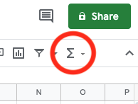
- On the toolbar, click the Functions button and choose SUM.
The beginnings of a SUM function appears in cell b10. Now we have to supply the argument, in this case, the range of cells containing the values we want to sum. - Point to the middle of cell b7, click and hold the primary mouse button and drag downward through cell b9, then release the mouse button.
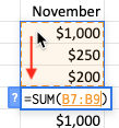
Selecting a cell or range of cells while composing a formula inserts a reference to that cell or range into the formula. - Press Enter/Return to commit the formula and see the result, $1,450.
Duplicate Formulas into Neighboring Cells
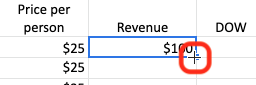
It is common to enter a formula into a cell and then wish to enter an identical formula in neighboring cells. Consider our SUM formula in cell B10. It would save time if we could copy the same formula into each cell of that row. Copy-and-paste would work, but there is another way to duplicate a formula into neighboring cells; drag the AutoFill handle, the small square on the bottom-right corner of the active cell, through the neighboring cells.
You can drag the Fill handle, pictured below, in any direction to copy the formula in the currently selected cell or to extend a series of labels, numbers or dates.
- With cell b10 selected, point to the AutoFill handle in its bottom-right corner, click and drag it to the right through column H, as shown below.
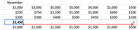
Sheets copies the formula from b10 into the cells to the right. The results show the total income for each month. Next, you will calculate total expenses for each month. - Select cell b16.
- On the toolbar, click the Functions button and choose SUM.
The beginnings of a SUM function appears in cell b16. - Point to the middle of cell b11, click and hold the primary mouse button and drag downward through cell b15, then release the mouse button.
- Press Enter/Return to commit the formula and see the result, $5,200.
Next you will total the Lessons income values. - Select cell i7.
- On the toolbar, click the Functions button and choose SUM.
- Click and drag from the middle of cell b7 through cell h7, and then press Enter/Return.
- If the Suggested autofill prompt appears, click the X to dismiss it without filling the formula down. I have other plans for this.
Now let's calculate the average earned each month from teaching our ski and snowboard lessons. - Select cell j7.
- On the toolbar, click the Functions button and choose AVERAGE.
- Click and drag from the middle of cell b7 through cell h7, and then press Enter/Return.
- Again, if the Suggested autofill prompt appears, click the X to dismiss it this time without filling the formula down.
Now let's AutoFill these two formulas down through the end of the list. We can do them both at once. - Select cells i7:j7.
- Point to the AutoFill handle in the bottom-right corner of the selected range of cells, click and drag it down through row 16.
The sums and averages for each income and expense row appear.
Simple Arithmetic Formulas
Not all formulas need a function like SUM or AVERAGE. To calculate profit or loss for each month, for example, the formula will simply subtract expenses from income. When writing formulas like these, keep in mind the following rules. All formulas:
- begin with an equal sign (=)
- may include the following symbols
+ Add - Subtract * Multiply / Divide ^ Exponent ( ) Do this first & Concatenate (append text) - may include references to cells on the current worksheet, or on other sheets in the current workbook. Referencing a cell that contains a value is smarter than typing the value itself into the formula, because if the value in a referenced cell changes, the formula result will update instantly to reflect the new result. To create a reference to a cell that lives on another sheet, click that sheet tab while writing the formula, and then click the cell.
- may include spaces around math symbols
- follow the arithmetic order of operations (PEMDAS)
- In cell b17, type an equal sign (=).
- Click on cell b10.
Sheets inserts a reference to cell b10 into your formula. You could have typed it yourself in uppercase or lowercase. - Type a minus sign (-).
- Click on cell b16.
- Press Enter/Return to commit the formula and see the result, $-3,750.
Now we will again duplicate two formulas at once. - Select cells b16:b17.
- Click and drag the AutoFill handle to the right through column I.
Calculate Percentage
Next, we will calculate a percent of total by dividing a part by the whole.
- On the Budget sheet, select cell k7.
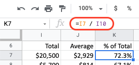
- Enter the formula =i7/i10 and press Enter/Return or Tab.
This formula divides the total revenue earned from teaching ski and snowboard lessons by the total of all three Income categories. The result of 0.7231040564 appears in cell k7. Let's format that cell to display this value in the percent style. - Select cell k7 again and then, on the toolbar, click the Format as percent button.

- To shave off one of the decimal digits, click the Decrease decimal places button. Repeat as desired.

Likewise, to add back more decimal digits, use the Increase decimal places button. - Use the AutoFill handle on cell k7 to copy the formula down into the next three cells, through row 10. Do not copy it to the end of the list, because only these first three totals are for Income categories. We will write a similar formula for the Expense categories next.
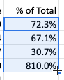
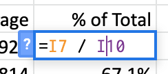
These results are obviously incorrect. How could the total income be 810% of itself? Let's inspect the formulas to see what went wrong. - Select cell k7 and then look in the Formula bar to remind yourself of the original formula.
- Move down one cell into k8 and inspect the formula there, which was the result of copying (or AutoFilling) the formula from k7.
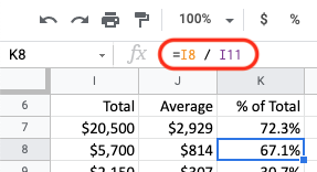
The copies of the formula are not identical to the original; we would not have wanted that! But the current results are not satisfactory either. This requires an understanding of relative referencing versus absolute referencing.
Relative vs Absolute References
- On the Budget sheet, select cell j7.
- Watch the Formula bar closely as you press Down Arrow to move down through the copies of this formula that we made earlier.
As we look at the formulas that Sheets wrote into cells j8:j16 when we AutoFilled, we notice that they are not letter-for-letter duplicates. It is a good thing, too! If they were, every formula result would be the same. Each formula seems to have magically adjusted to its new location.
J 6 Average 7 =AVERAGE(B7:H7) 8 =AVERAGE(B8:H8) 9 =AVERAGE(B9:H9) 10 =AVERAGE(B10:H10) 11 and so on...
The magic is not in the duplicating process, but in the way we referenced the range of cells when writing the original formula. The formula in cell j7 refers to cells b7 through h7 using relative referencing. It thinks of them as the range of cells beginning eight cells to my left through two cells to my left.
When Sheets copies that logic into a new location, the relative references point to different cells because they started from different cells. Relative referencing makes it possible to copy formulas and have them work properly in their new context.
Relative referencing is the default referencing style. That is, when writing formulas, clicking a cell produces a relative reference. However, relative references are not appropriate in all instances. If a formula refers to a cell for a specific purpose, and every copy of that formula should refer to the same cell, we should refer to that cell using absolute referencing rather than relative referencing.Absolute references treat references to cells as a specific location in the worksheet, rather than the location that is x columns and y rows away from the formula cell. Compare this to giving directions to a friend you wish to meet for lunch. You could tell them “From where you are now, go south two blocks, turn left, and it is the third door on the right.” Or you could give them the address of the restaurant, so that no matter from where they begin, they will find the correct location.
To create an absolute reference, put a dollar sign ($) in front of both the column letter and the row number of a cell reference, as in $D$12. The function key F4 is a convenient shortcut for changing referencing styles, as described in the next exercise.
- Look again at the formulas in cells k7 through k10.
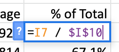
See the pattern? Relative referencing caused our reference to i10 in the original formula to slide down to i11, i12, and i13 in the duplicates. Using an absolute reference to i10 would have made Sheets point specifically to that cell in each copy, rather than pointing to its location relative to the new starting point. - Double-click cell k7 to edit its formula.
- Click in the i10 part of the formula.
- Press the function key F4 key on the keyboard.
Sheets adds dollar signs to the cell reference. The formula now reads =I7/$I$10.
- Press Enter/Return to commit the changes to the formula.
The result is the same, of course, but the behavior when we copy or AutoFill the formula will improve. - Select cell k7 and use the AutoFill handle to copy the revised formula down through cell k10, overwriting the existing entries.
The results are now correct. If you inspect the copies of the formulas, you will see that each copy divides by cell i10 because we referred to that cell using an absolute reference.
Determining Which Referencing Style to Use
To determine which referencing style to use, ask yourself two questions every time you write a formula:
- Am I going to copy this formula anywhere? If no, then just use the default relative referencing, because it does not matter. If yes, however, then ask…
- Are there any cell references in this formula that should not change from copy to copy? Those are the references that need dollar signs.
Now let’s get some more practice with absolute references.
- In cell k11, write a formula that divides total payroll expense by the total of all expenses: =i11/i16
- Knowing that you are going to copy it down through the other expenses, make the reference to i16 absolute by adding dollar signs (remember the F4 keyboard shortcut). The formula should now read =i11/$i$16
- Press Enter/Return to commit the formula.
- Copy the formula down through cell k16.
This time, the copies of the formula perform perfectly; we avoided making the referencing mistake by asking ourselves those two simple questions. Make that a habit in your own spreadsheet work.
Concatenate and Parse Text
Concatenation is a long word that means to combine strings of text characters together to make a longer string. There are two ways to concatenate text in Sheets: the ampersand symbol (&) or the CONCATENATE function. The ampersand symbol is easier and equally effective, so we will use it.
- Navigate to the Staff sheet.
- In cell d14, write the formula =c14 & b14 and press Enter/Return to commit the formula.
The result is correct, but not pleasing. Note that spaces around operator symbols like & are optional, not required; I include them because they make the formula easier to read and debug.
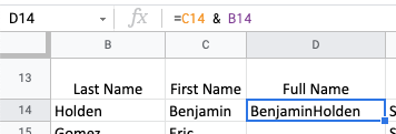
Now we will add a space in between the first name and last name. We must enclose strings of characters we want included in the result in double quotation marks; even a character as insignificant as a space. Otherwise, Sheets will assume that we are adding space into the formula to make it more readable. Similarly, we would enclose literal words or phrases that we want included in formula results in quotes so that Sheets would know that they are not cell references, function names, or cell range names. - Edit cell d14 to include a space between first and last name, like this: =c14 & " " & b14
- Press Enter/Return to commit the changes to the formula.
- Use AutoFill to copy the formula in d14 down through the end of the list. (Hint: double-click the AutoFill handle.)
Parse Text
To parse text means to extract a piece of the text; parsing is the opposite of concatenation. There are several functions that parse text, including LEFT, MID, and RIGHT. The LEFT function returns characters from the beginning (the left side) of a text string. The MID and RIGHT functions return characters from the middle and end of a given text string respectively, and all three return a result that is a text string.
In cell o14, let’s write a formula to return the ZIP code from the Hometown in cell L14.
- Select cell o14, then type an equal sign, followed by the first few letters of the RIGHT function: =ri
As you type, a hint menu displays the names of functions that Sheets thinks you may be trying to include in your formula. Use the Down and Up arrow keys to select a function, and the Tab or Enter/Return key to insert the selected function into the formula. - When the RIGHT function is selected in the hint menu, press Tab to insert it into the formula.
- To get help with a function, click the Expand details icon.
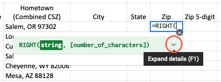
The RIGHT function returns x number of characters from the end (the right side) of a text string. Likewise, the MID and LEFT functions return the specified number of characters from the middle or beginning of a given text string, returning a text result. The RIGHT function has one required argument, the source string of text from which we want to get the substring, and one optional argument, the number of characters to grab. - Click on (or type a reference to) cell L14.
- Type a comma.
Functions use commas to separate arguments. - Type the number 5 as the number of characters to grab, since all the ZIP codes are five characters in length.
- Type a closing right parenthesis ) character. The formula should now read =RIGHT( L14, 5 )
- Press Enter/Return to commit the formula.
The formula returns the result of 97302, the ZIP code of Salem, Oregon, my hometown. - Drag the AutoFill handle in cell o14 down through cell o21.
Extracting text is simple enough, right? The tricky part is that in most cases, the number of characters you want to grab is different for each instance of the data, i.e., city names are not all the same length. That is where the SEARCH function comes into play.
SEARCH function
The SEARCH function searches through a text string for a specified character or string of characters. If it does not find it, it returns an error. If it does find it, it returns the character position of the first instance. For example, in the text string John Smith, if we told the SEARCH function to look for the letter H, it would return the number 3, because the first instance of an H is in the third character of the string. Note: SEARCH is not case-sensitive.
Let’s see how the SEARCH function works on its own, then we will nest it inside the LEFT function to return the City names from the Hometown data.
- On the Staff sheet, in cell n14, write the following formula: =SEARCH( "," , L14 )
This formula searches for a comma "," in cell L14 and returns the character position of the first one it finds. If it does not find one, it returns a #VALUE error.
This formula may at first look confusing because of the commas. The first comma is enclosed in quotes; that is our search term, or the needle. The second comma is the separator between the two arguments. Lastly, L14 is the text to search, or the haystack. - Press Enter/Return to commit the formula.
The formula returns the result of 6, the position of the first comma in the hometown of Salem, OR 97302. - AutoFill the formula in cell n14 down through cell n21.
Each hometown may have a comma in a different character position, depending on the length of the name of the city, so the results vary. One thing we know for certain; the number of characters in each City name is one less than the character position of the comma. Therefore, if we search for the comma and then subtract one from that result, we will get the length of the City name. Let’s write that formula in cell m14. - In cell m14, write the following formula: =LEFT( L14, SEARCH( "," , L14 ) - 1 )
- AutoFill the formula in cell m14 down through cell m21.
- Select cells n14:n21 and press the Delete key on the keyboard to clear those cells.
We’ll save the State column as a lab exercise if there is time left over.
IF for Conditional Logic
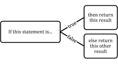
Logical (or conditional) functions let us build branching logic into our formulas. Most follow the pattern if-then-else; like this:
Let’s use conditional logic to automate the Price column on the Lessons sheet.
- Navigate to the Lessons sheet.
- Select cell h23.
- Type =if and the press Enter/Return.
- Complete the formula as follows: =if( f23 = "Group", $c$5, $c$6 )
This formula evaluates the expression f23 = "Group". If that statement is true, then it returns the value presently in cell c5, our price per person for Group lessons. If it is false, it returns the value in c6, our price per person for Private lessons. - Press Enter/Return to commit the formula.
The formula returns the result of 25. - AutoFill the formula in cell h23 down through the end of the list by double-clicking the AutoFill handle. (Hint: If it will not AutoFill, then clear the cells in column H below the formula and then try the AutoFill again. A shortcut to select from the current cell to the end of a list is Control + Shift + Arrow Key in the direction you wish to go.)
- Change the prices in cells c5 and c6 and observe the effect on the Price per person formula results.
We could also have accomplished this same feat using the VLOOKUP function, which you will learn next.
VLOOKUP for Performing Lookups
The VLOOKUP function searches the first column of a table until it finds a specified lookup value or the closest match, then it marches across that row a specified number of columns to return the value in that cell. As an analogy, at the checkout counter of a store, the clerk scans the barcode of a product, which begins a VLOOKUP of their Products table. When it finds that product’s ID code in the database, it marches over to the Price column and returns the price.
The HLOOKUP function works the same way, but transposed ninety degrees. It searches across the first row of a table until it finds the lookup value or the closest match, then marches down a specified number of rows and returns the contents of that cell.
Here is a close look at the syntax of the VLOOKUP function:
=VLOOKUP( search key, range, column index number, is sorted )
| search key | the value to search for, i.e., the needle |
| range | the range to search through, specifically, its first column, i.e., the haystack |
| column index number | if the search key is found in a row of the range, this number specifies from which column to return a value, where the first column in the range is column index number 1. |
| is sorted (optional) | you should specify TRUE or FALSE. If you leave it blank, it uses TRUE by default. If searching for the closest match to search key is satisfactory, then use TRUE, but if you require an exact match, use FALSE. To use TRUE successfully, the range must be sorted by the values in its first column. |
Let’s write a formula to return the full name of the staff member who taught each lesson. We have the employee ID number of the instructor in column D, so we can use it to find their row in the employee list on the Staff sheet and retrieve their full name.
- On the Lessons sheet, select cell e23.
- Type =vl and press Enter/Return.
- Click cell d23 to use as the search key.
- Type a comma character to separate the first argument from the next.
This second argument is range, the list of data to search and, hopefully, retrieve the desired value. Our range is on the Staff sheet, so we will jump there to refer to the cells that contain the list of employees. - Click the Staff sheet tab.
- Click and drag from cell a14 through cell p21 to insert a reference to that range of cells into the formula.
- Press the function key F4 to change the referencing style for this range to absolute.
We know that we are going to copy this formula a thousand times. Since this list of employees does not move relative to the formula cell in Lessons, we will fix this reference so it does not adjust. - Type a comma character to separate this argument from the next.
- If you cannot see column A of the Staff sheet, scroll back to the left until you can. Counting from the first column of the range that you just selected, which column contains the Full Name value we want to return? The fourth column; so type the number 4 as the index argument.
- Type one last comma to separate this argument from the last.
Our employee list happens to be sorted by its first column, but if it were not, we would still want to retrieve the full name of the employee whose ID number matches the search key value from the Lessons list. We are looking for an exact match, not the closest value not exceeding our search key. Thus, we will specify FALSE for the is sorted argument. - Type FALSE in upper or lowercase characters, and not enclosed in quotes.
TRUE and FALSE are logical values in Sheets, not string literals. - Type a closing right parenthesis ) character.
The formula should now read =VLOOKUP( D23, Staff!$A$14:$P$21, 4, FALSE ) - Press Enter/Return to commit the formula.
The formula returns the result Eric Gomez, who has employee ID 0002 on the employee list of the Staff sheet. - AutoFill the formula in cell e23 down through the bottom of the Instructor name column.
Now that you know what VLOOKUP can do, let’s use it a few more times, on the Customers sheet. - Navigate to the Customers sheet.
- In cell d5, write a VLOOKUP formula to return the First name of the customer whose ID is in cell d4.
=VLOOKUP( $d$4, $a$10:$k$76, 2, FALSE ) - Copy that formula down through the next two cells.
- Edit the index argument of each copy of the formula so it returns the Last name and the Preference values, respectively.
- In cell d4, type 108 and press Enter/Return. The lookup functions should now return values about Sonia Long.