Chapter 1: Format Cells in Google Sheets

In this chapter, you will learn how to:

upload, open, and convert Excel files into Sheets files
format numbers and dates
apply conditional formatting to cells

Google Sheets is the spreadsheet app in the Google Suite. Similar to Microsoft Excel, it lets you create and share spreadsheets containing text, numbers, calculations, lists of data, and charts.

Upload, Open, and Convert Excel Files

There is an Excel file that we will use as a starting point for the exercises in this class. Let's upload it into your Google Drive and then save a copy of it as a native Google Sheets file.

Launch a web browser and go to drive.google.com
Create a new folder in your Google Drive called Class Files.
Double-click the new Class Files folder to navigate into it.
Upload the Excel file we provided into the Class Files folder of your Google Drive.
Once uploaded to your Google Drive, double-click the Excel file there to open it.
It will open into a separate browser tab.
If a Welcome to Office Editing message appears, close it by clicking the X in its top-right corner.
Even though Google Sheets can now edit native Excel files, we are going to convert this file into a native Sheets file.
On the menu bar near the top of the Google Sheets interface (not your web browser's menu bar), click File > Save as Google Sheets.

The copy will open into its own browser tab.
Close the browser tab containing the Excel version of the file. We will henceforth work with the Sheets version.
If needed, switch back into the browser tab containing the Powder Day Google Sheets file.

Format Numbers

You use numeric values for many purposes: quantities, dollars, percentages, dates. Without formatting, however, all values look the same. Sheets makes it easy to apply appropriate number formatting for all common uses of numeric values.

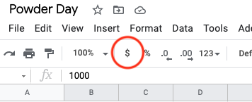
In the Budget sheet, select cells b7:j17.
On the toolbar, click the Format as currency button.

The numbers take on a different appearance. There are other number formats from which to choose.
On the toolbar, click the More number formats menu and try Accounting, and then apply Currency (rounded).

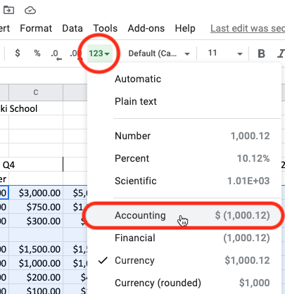
Please note that even the empty cells are now formatted with the Currency (rounded) format, despite not containing any numbers to manifest the formatting. Later, when we write formulas into these cells, the formatting will already be there.
On the sheet tabs at the bottom of the window, click the Inventory sheet.
Select cells k9:l16.
Apply the Currency number format to these cells.
We would not want to use Currency (rounded) here because at least one of the numbers has cents that we would want to appear. See what happens when you apply Currency (rounded) here. The numbers are rounded to the nearest whole number, but the rounding is only for display purposes; the accurate number is still stored in the cell.

Format Dates

Spreadsheet and database programs treat dates as numbers; the number of days elapsed since some starting date. Google chose 12/31/1899 as Sheet's starting date, its day number 1. Every day after that gets the next higher day number. Because a date is just a number, you can use dates in math formulas. However, to make date numbers meaningful to us humans, we format them to look like dates. Sheets handles this automatically, sensing when we enter a date and first converting it to the corresponding day number, and then applying a simple date format to the cell. However, we can choose from many fancier date formats.

Select the Acquisition Date cells in f9:f16.
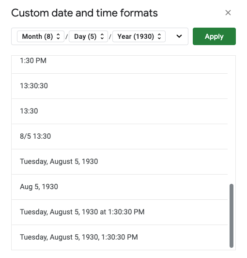
On the toolbar, click the More number formats menu and choose Custom date and time.
From the scrollable list of date and time formats, choose a format you like and click Apply.
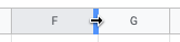
You may need to widen the column to display the dates fully. Double-click the border between column headers F and G.
Navigate to the Staff sheet of the workbook.
Select cells f14:f21.
Holding down the Control key (Windows) or Command key (Mac), select these additional ranges: h14:h21 and j14:j21.
These additional cells are empty now, but they will eventually hold dates, so formatting them now will save us from having to do it later.
On the toolbar, click the More number formats menu. Near the bottom of the menu, the date format(s) you have applied recently appear; choose one to apply it to the selected cells.
If necessary, widen column F to show the dates fully.

Apply Conditional Formatting

Conditional formatting lets you spot trends, patterns or outliers in your lists or ranges of data. You apply one or more formatting rules to a range of cells. A rule consists of a conditional statement that is either true or false for each cell in the selected range, and a corresponding format. In each cell for which a condition is true, the format applies to that cell.

Navigate to the Lessons sheet of the workbook.
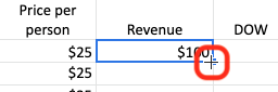
In cell i23, write the formula =g23*h23 to calculate the revenue generated by this first group ski lesson.
When you press Enter/Return, Google Sheets may prompt you to autofill the formula to the end of the list. Please have it do so.
If it does not prompt you, autofill the formula down manually by double-clicking the AutoFill handle in the bottom-right corner of the cell.
With cell i23 selected, on the keyboard, press Ctrl + Shift + Down Arrow to select through the bottom of the Revenue column of data.
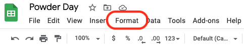
With cells i23:i1022 selected, click Format > Conditional Formatting on the menu bar.
The Conditional format rules pane appears on the right side of the window.

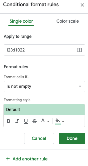
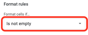
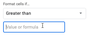
There are two tabs, or panels, in this pane: Single color and Color scale. Use Single color to draw attention to cells that meet specific conditions. Use Color scale to compare all the values in the range of cells to each other, as in a heat map.
On the Single color tab, click the menu just below the prompt Format cells if... and choose Greater than.
In the Value or formula field that appears, type 220.
Below the Formatting style heading, click Default and select a formatting style you like.

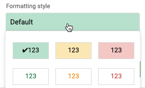
You may manually apply formatting attributes to the conditional formatting rule also or instead using the icons below the Default style menu.
Click Add another rule near the bottom of the Condtional format rules pane.
In the new rule, specify to Format cells if... Less than and then specify 100 in the Value field, and choose a red Formatting style.
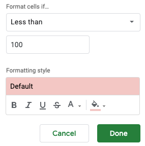
Click the Done button when finished defining conditional format rules for the selected range of cells.

The Conditional format rules pane remains on the screen until you close it or close the file.
To edit the condition or formatting of a rule, click the rule once, make the changes, and click Done.
To remove a conditional format rule, click the Remove rule trash can icon that appears when you point to that rule.
Close the Conditional format rules pane.