Chapter 5: Google Sheets
In this chapter, you will learn how to:
- create spreadsheets
- enter data and simple formulas
- manage lists of data
- save to your Google Drive
Google Sheets is the spreadsheet app in the Google Suite. Similar to Microsoft Excel, it lets you create and share spreadsheets containing text, numbers, calculations, lists of data, and charts.
Create Spreadsheets
To launch Google Sheets and create a new spreadsheet:
- Launch a web browser and go to google.com or any app in the Google Suite.
- Click the Google apps button, scroll down through the gallery of apps, and click Sheets.
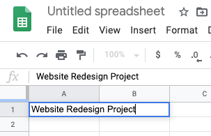
The Google Sheets home page appears, usually in its own tab, showing several templates to help jump-start your work. To see more templates, click Template gallery. - Click the Blank template to create a new, empty document, or another template to use it as the starting point for your new document.
A new document appears.
A Google Sheets spreadsheet file consists of one or more sheets. A sheet, like an accountant's ledger paper, is made of columns and rows. Initially, a sheet contains 26 columns and 1000 rows, but you may add more of each as needed. You may also create new sheets as needed within the same spreadsheet file, and of course, you may create as many spreadsheet files as your allotted space on Google Drive can hold.
The intersection of a column and a row is a cell. Each cell's address is set by its column letter and row number, as in A1 or Z1000. There is always one active cell, which has a blue border around it. Click on a cell to make it the active cell. You may also use the keyboard to move between the cells.
| To move | Press |
|---|---|
| Down | Enter/Return, or Down Arrow key |
| Up | Shift + Enter/Return, or Up Arrow key |
| Right | Tab, or Right Arrow key |
| Left | Shift + Tab, or Left Arrow key |
Enter Data and Simple Formulas
To make an entry into a cell:
- Select a cell to make it the active cell.
- Type or paste the entry.
- Press Enter/Return or Tab to commit the entry and move to the next cell.
If an entry extends into its neighboring cell(s), it will still display properly if those cells are unoccupied. If needed, you can widen the column, discussed later.
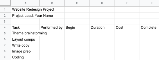
Make the following entries into Sheet1.
Changing column width
To change the width of a column, point to the border between it and the column header to its right, as shown below.
![]()
You can either:
- click and drag to manually set the width, or
- double-click to set the width automatically to the column's best fit (based on its widest entry)
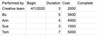
Make these additional entries:
Writing formulas
You write formulas into cells to return calculated results. Formulas use familiar arithmetic symbols like + and - for addition and subtraction, asterisk (*) for multiplication and slash (/) for division. You can also use built-in functions like SUM, AVERAGE, and others, to write complex expressions.
Let's write a formula to return the sum total of days in the Duration column by summing the values in cells d5 through d9.
- Select cell d10.
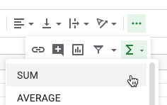
Always begin a formula by selecting the cell where the result should appear. - On the toolbar, click the Functions button and choose SUM.
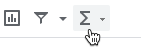
If the Functions button is not visible on the toolbar, click the ... (More) button to reveal the additional tools, then click Functions, then SUM.
- If an informative pane appears, click the Close button in its top right.
- Drag from cell d5 down through cell d9 and release.
This causes the cell range d5:d9 to be entered as the argument of the SUM function.
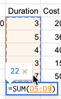
- Press Enter/Return to commit the formula and see the result.
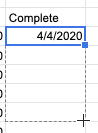
Next, let's calculate the Completion date of the first task by adding its Duration (number of days to complete that task) to its Begin date.
- Select cell f5.
- Type an equal sign (=).
Every formula begins with an equal sign. - Click on cell c5.
- Type a plus sign (+).
- Click on cell d5.
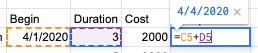
- Press Enter/Return to commit the formula.
Finally, let's calculate the Begin date of all the other tasks by having them start one day after the Complete date of the prior task.
- Select cell c6.
- Type an equal sign (=).
Every formula begins with an equal sign. - Click on cell f5.
- Type a plus sign (+) followed by the number one (1).
- Press Enter/Return to commit the formula.
Filling formulas
You can replicate a formula into its neighboring cell(s) to place the same kind of formula in it by dragging its Fill handle. Let's copy the formula we used to sum the Duration column into the empty cell to its right. The result will sum the Cost values.
- Select cell d10.
- Click and drag the Fill handle, shown below, to the right through cell e10.
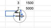
The resulting formula sums cells e5:e9.
In the same way, let's use the Fill handle to replicate the formula in cell f5 down through the end of the list of tasks.
- Select cell f5.
- Click and drag the Fill handle down through f9.
Some of the formulas return incomplete results because the cells they refer to are still empty. However, as soon as we fill those cells, these formulas will return good results. Lastly, let's replicate the calculation of Begin dates down through the end of the tasks list.
- Select cell c6.
- Click and drag the Fill handle down through c9.
The Begin date is calculated to be the date after the Complete date of the previous task. In this way, all the task dates are dependent upon the first task's Begin date. If it changes, all the other dates will change accordingly.
- Double-click in cell c5.
- Change the date to April 3, 2020.
All the other dates change as a result of this change, as they are all calculated from this value either directly or indirectly.
Manage Lists of Data
With Google Sheets, you can sort and filter long lists of data. You can also import data from other files, including Excel workbooks.
Import Excel data
- Click the File menu and choose Import.
- In the Import File dialog, click the Upload tab, and then click the Select a file from your device button.
- Navigate to the folder containing your class files and open Trips.xlsx.
- For the import location, choose Insert new sheet(s).
- Click Import data.
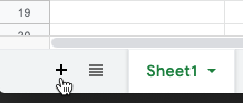
The data from the Excel sheet is copied into a new sheet in the current spreadsheet file. If you ever need to create a new sheet from scratch, just click the Add Sheet button.
Selecting ranges of cells
Before you can perform a sort or many other actions in Sheets, you must select the range of cells you wish to affect. There are many efficient ways to select ranges of cells.
| To select | Do this |
|---|---|
| any range of cells | Point into the center of the first cell of the range and then click and drag to the last cell, or Click the first cell of the range to select it, and then while holding down the Shift key, click the last cell of the range |
| From the current cell in any direction | Hold the Shift key down while pressing any Arrow key |
| a range of occupied cells | Select one of the corner cells of the occupied range, and then, holding the Control and Shift keys down (on Mac or Windows), press an Arrow key in the direction you wish to select. Do it again, if necessary, for the next direction, i.e., Ctrl+Shift+Down Arrow, then Ctrl+Shift+Right Arrow.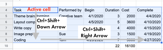 |
| Entire column | Click the column header letter |
| Entire row | Click the row header number |
Sorting data
- On the Trips sheet, select cells a1:h41.
- Click the Data menu and choose Sort range.
- In the Sort range dialog box that appears, check the box Data has header row.
- Click the pop-up menu and specify to sort by Project from A to Z.
- Click the Add another sort column button.
- Use the new pop-up menu to specify Team Member as the secondary sort field, from A to Z.
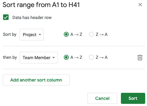
- Click the Sort button to sort the rows.
The list is now sorted first by Project and then by Team Member.
Filtering data
Filtering data hides rows that do not meet your criteria, so you can bring to the surface only that which you need to see, but then easily restore the hidden data to show everything again.
- If your list does not have a header row of column/field labels, create one.
- Select any one cell in the list to filter.
- Click the Data menu and choose Create a filter.
Filter menu icons appear in the header row of your list.
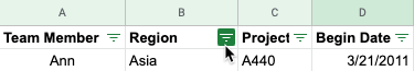
- Click one of the filter menu icons and specify your filter criteria. You may filter by color, condition statement, search values, or by checkmark.
- Click OK to apply the filter.
Only the rows that meet your criteria remain visible. All the other rows are hidden. To restore the list to its original unfiltered state, click the Data menu and choose Turn off filter.
Save to your Google Drive
Relax! Your spreadsheet file is already saved. Google Sheets saves your work for you automatically during idle time. However, you should probably give your files better names.
To save (rename) the current Google Sheets spreadsheet file:
- Click in the spreadsheet title field at the top left of the window.
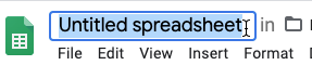
- Type a new name, Class Exercises, and press Enter/Return.